PMA Analysis
This document describes how to configure the PMA (Performance Measurement and Attribution) analysis.
The PMA analysis allows viewing investment returns, absolute and relative to a benchmark, over a period at any level of the portfolio structure, in order to provide an understanding of the source of the return.
Note that PMA analysis is the newer version of the legacy Performance Measurement analysis. It is recommended to use PMA as it offers the following improvements over Performance Measurement:
| • | The PMA architecture (time series based data and its own database) simplifies debugging the process, and offers an historical view of the data behind the final reports. |
| • | PMA offers the possibility to use multiple benchmarks, improving the sources of comparison against your portfolios. |
| • | The formula-based column variables allow end users to clarify the underlying figures' definitions by viewing them in the Portfolio Workstation. |
| • | Any specific performance measure or custom report required for your local operations can be configured as the formula-based columns provide the flexibility to define new variables. |
The PMA analysis requires several analyses and scheduled tasks to be run as prerequisites. They are, in the following order:
| • | Official P&L analysis |
| • | EOD_OFFICIALPL scheduled task |
| • | Investment Indicators analysis |
| • | PMA Daily analysis |
| • | AM_PMA_EOD scheduled task |
| • | PMA Period analysis |
| • | PMA analysis |
1. Before You Begin
In order to run a PMA analysis, you must first configure the following:
| • | Install the Analysis Time Series API optional module. It is required in order to use the PMA analysis. |
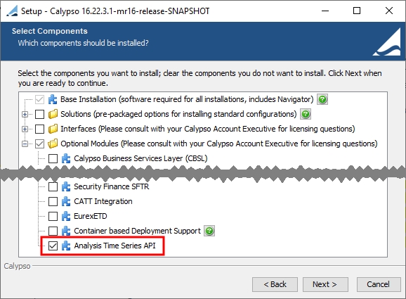
 Please refer to the Calypso Installation Guide for complete details.
| • | Make sure that the Buy Side Data Warehouse database is configured - See Buy Side Data Warehouse for details. |
| • | The Time Series server must be running. It saves the PMA daily results in the database. You can start it from the following location, or from the Calypso DevOps Center. |
<calypso home>/deploy-local/<Environment>/calypsoservicestimeseriesserver.bat\.sh
Please refer to the Calypso Installation Guide for details on using the Calypso DevOps Center.
| • | A Position Specification with a Strategy key as an additional liquidation property (recommended). |
| • | An "Official" P&L Configuration with Investment P&L measures. |
You also need to run the Official P&L analysis for the "Official" P&L Configuration.
Sample configurations are shown below.
Please refer to Calypso Official P&L documentation for complete details.
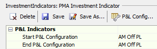
| • | An Investment Indicators analysis. The Investment Indicators analysis must use the same Official P&L configuration used to generate the portfolio Official P&L marks and positions. |
See Investment Indicators Analysis for details on configuring an Investment Indicators analysis and its prerequisites.
| • | A PMA Daily analysis. |
See PMA Daily Analysis.
| • | Portfolio and benchmark PMA figures historized as time series. |
See AM_PMA_EOD Scheduled Task.
| • | A PMA Period analysis. |
See PMA Period Analysis.
| • | Analysis Server Configurations for the PMA Daily, PMA Period, and PMA analyses. |
See Portfolio Workstation for details on defining Analysis Server Configurations.
1.1 Buy Side Data Warehouse
The Buy Side Data Warehouse is a database separate from the core database that allows storing long term Official P&L data for faster computation.
Set the following environment properties for the Buy Side Data Warehouse:
| • | BuysideDataWarehouseDRIVER=<database driver> |
| • | BuysideDataWarehouseDBURL=<database URL> |
| • | BuysideDataWarehouseDBUSER=<database user> |
| • | BuysideDataWarehouseDBPASSWORD=<database password> |
Please refer to Calypso Database Administration documentation for details on creating a new database.
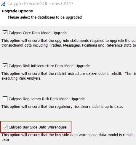
NOTE: If you are using Buy Side Data Warehouse, make sure that you run Execute SQL with "Calypso Buy Side Data Warehouse" checked so that the database can be properly upgraded as needed.
1.2 Position Specification
It is recommended to use a Position Specification with a Strategy key as an additional liquidation property.
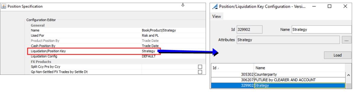
See Computing Asset Management Positions for complete details.
1.3 P&L Configuration
Sample "Official" P&L Configuration
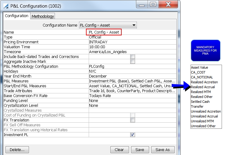
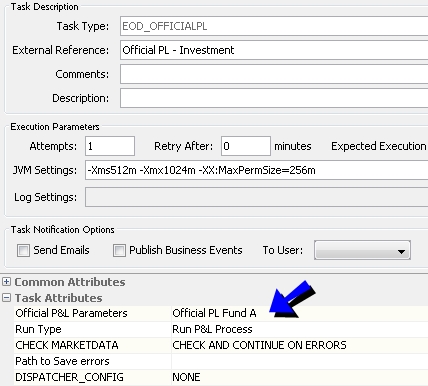
Sample Official P&L parameters for the "Official" P&L Configuration
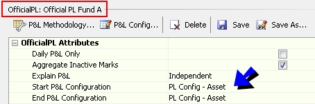
Then run the scheduled task EOD_OFFICIALPL for the Official P&L parameters.
Ⓘ [NOTE: The position spec used to run the scheduled task (in the trade filter) should be the same as the position spec used to run the Portfolio Workstation analysis (in the Analysis Server Configuration trade filter template).]
2. Configuring the PMA Daily Analysis
The PMA Daily analysis is based on the Active analysis so the benchmark and active portfolios have positions reflecting the difference between the portfolio and the benchmark.
See Active Analysis for more details on the Active analysis.
The PMA Daily results are historized by a scheduled task over a period defined in the PMA analysis without the need to run the task every business day. The task is executed for every period selected in the Period Config parameters of the PMA analysis.
The PMA Daily report shows single-period performance and attribution indicators. It is necessary to configure the PMA Period and PMA analyses and run the AM_PMA_EOD scheduled task to consult a consolidated multi-period output. The PMA Daily intention is to explore the structure of a single-period report as a preview of the final analysis.
From the Calypso Navigator, navigate to Configuration > Reporting & Risk > Analysis Designer.
Right-click a PMA Daily folder, and choose "New Analysis" to configure the parameters. You will be prompted to enter a configuration name.
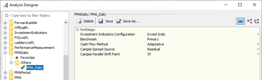
| » | Enter the fields described below as needed, then click Save. |
Settings
|
Indicators |
Description |
|---|---|
|
Investment Indicators Configuration |
Select an Investment Indicators analysis parameter.
The Investment Indicators analysis must use the same Official P&L configuration used to generate the portfolio Official P&L marks and positions. The dedicated Investment Indicators must have an EOD P&L configuration as PMA uses EOD P&L Marks to generate historical time series data:
|
|
Benchmark |
Select which benchmark(s) to compare the portfolio to: Primary and/or Secondary as defined at the fund configuration or portfolio hierarchy level. A fundamental function of the PMA analysis is the flexibility to select multiple benchmarks as references.
|
|
Cash Flow Method |
Select the daily cashflow adjustment: Beginning of the day, End of the day, or Adaptive. If Adaptive is selected, depending on the sign of the position (long/short) and the trade sign (buy/sell), the cashflows are either considered at the beginning of the period or at the end of the period. |
|
Select the Spread calculation logic: Residual or Benchmark Sector.
|
|
|
Select the curve point to use for calculating the Shift effect.
|
The Cash Flow Method, Campisi Spread Source, and Campisi Parallel Shift Point parameters determine some of the formula-based columns.
Once the columns are imported into the Portfolio Workstation, you can view the column formula definitions. It is also possible to modify the formula-based columns using Pricing, Market, or Risk Indicators from the source analysis to create custom definitions for a PMA report.
The formula-based column variables allow end users to clarify the underlying figures' definitions by viewing them in the Portfolio Workstation.
Any specific performance measure or custom report required for your local operations can be configured as the formula-based columns provide the flexibility to define new variables.
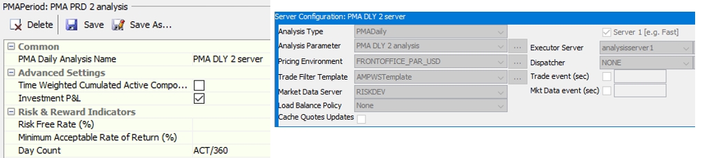
At this point you may wish to create the Analysis Server Configuration for the PMA Daily analysis.
See Portfolio Workstation for details on defining Analysis Server Configurations.
3. Running the PMA Daily Analysis
To execute a PMA Daily analysis, select an ad-hoc valuation date. The selected date should be at least two days after the portfolio's OPL inception date. For non-portfolio benchmarks, the first record date should be congruent with the OPL inception date of the linked investment vehicle.
4. Configuring the PMA Period Analysis
The PMA Period analysis is simply responsible for fetching historized PMA Daily analysis data for a given period.
While the PMA Period analysis can be viewed in the Portfolio Workstation for investigation purposes, it is not meant to be used for reporting in and of itself.
From the Calypso Navigator, navigate to Configuration > Reporting & Risk > Analysis Designer.
Right-click a PMA Period folder, and choose "New Analysis" to configure the parameters. You will be prompted to enter a configuration name.
| » | Enter the fields described below as needed, then click Save. |
Common
|
Indicators |
Description |
|---|---|
|
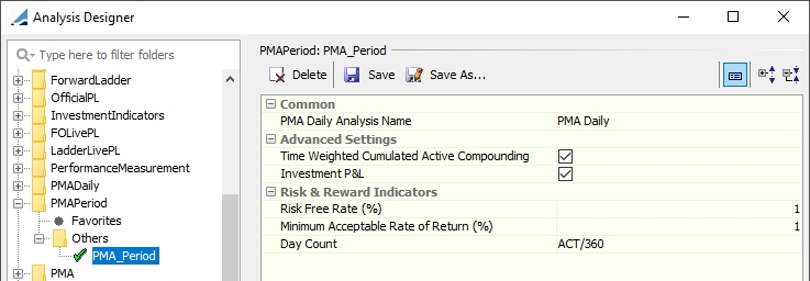
PMA Daily Analysis Name |
Select a Analysis Server Configuration which has been defined for a PMA Daily analysis.
|
Advanced Settings
|
Indicators |
Description |
|||||||||||||||
|---|---|---|---|---|---|---|---|---|---|---|---|---|---|---|---|---|
|
Time Weighted Cumulated Active Compounding |
Check to compute cumulated active return with geometric return formula on the daily active return, or leave un-checked to compute it as the difference between the cumulated portfolio return and benchmark return. |
|||||||||||||||
|
Investment P&L |
When selected, the Cumul Return Cross is computed from Cumul Return FX and Cumul Return Local, like Investment P&L breakdown.
|
Risk & Reward Indicators
|
Indicators |
Description |
|---|---|
|
Risk Free Rate (%) |
Enter the annualized risk-free rate over the period. |
|
Minimum Acceptable Rate of Return (%) |
Enter the minimum acceptable rate of return. Used for upside/downside deviations and Sortino ratio. |
|
Day Count |
Specify the day count normalization for risk indicators. |
At this point you may wish to create the Analysis Server Configuration for the PMA Period analysis.
See Portfolio Workstation for details on defining Analysis Server Configurations.
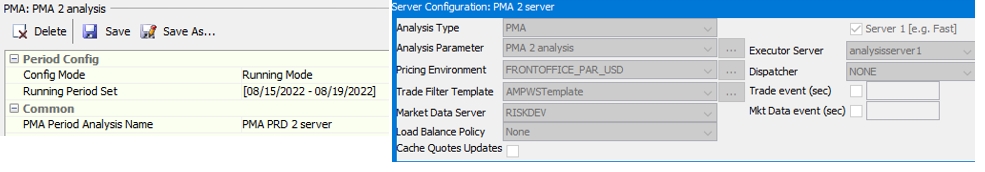
5. Configuring the PMA Analysis
From the Calypso Navigator, navigate to Configuration > Reporting & Risk > Analysis Designer.
Right-click a PMA folder, and choose "New Analysis" to configure the parameters. You will be prompted to enter a configuration name.
| » | Enter the fields described below as needed, then click Save. |
Period Config
|
Indicators |
Description |
|---|---|
|
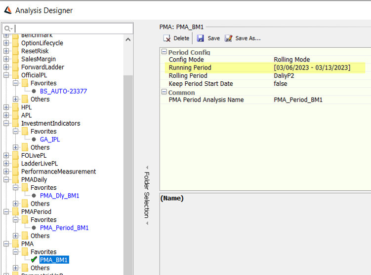
Config Mode |
Select Running Mode or Rolling Mode. Running Mode allows defining one or several running periods (MTD, YTD, etc.) and custom periods (date ranges). Rolling Mode uses a running period and also adds a rolling decomposition of the period (weekly, monthly, etc.). For example, you can have a YTD period sub-divided into monthly periods. |
|
Rolling Period |
If Rolling Mode is used, select a date rule (weekly, monthly, etc.). You can click Period Date Rule to define a new date rule as needed. |
|
Running Period |
List of observation periods used to compute and aggregate effects (YTD, MTD, custom, etc.). You can select a date rule from the list, then click >> to add it. You can click Period Date Rule to define a new date rule as needed. You can specify a custom period, then click + to add it. |
|
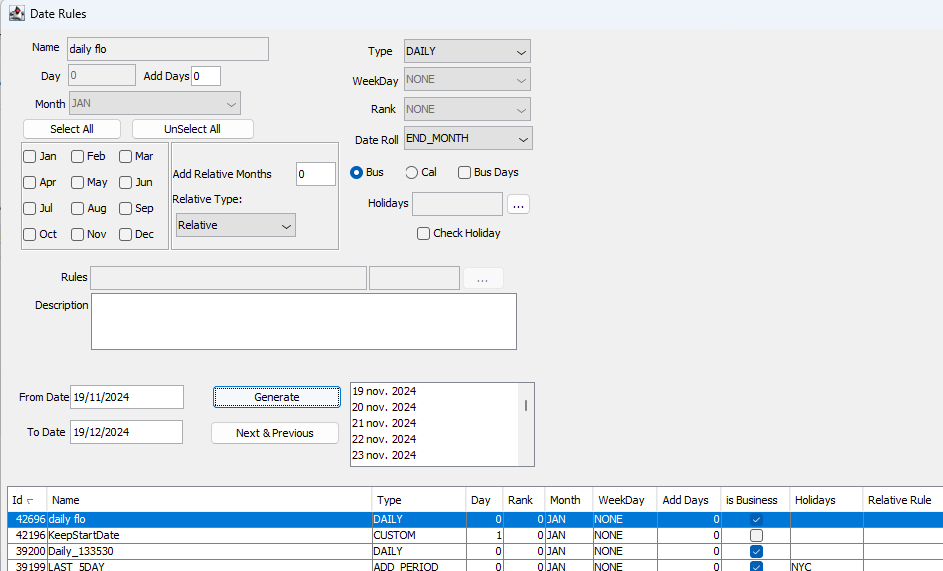
Keep Period Start Date |
The default value for Keep Period Start Date field is false. To activate sliding period, Keep Period Start Date field should be set to true and define a DateRule Daily like this (type DAILY):
|
Common
|
Indicators |
Description |
|---|---|
|
PMA Period Analysis Name |
SSelect an Analysis Server Configuration which has been defined for a PMA analysis.
|
At this point you may wish to create the Analysis Server Configuration for the PMA analysis.
See Portfolio Workstation for details on defining Analysis Server Configurations.
6. Running the AM_PMA_EOD Scheduled Task
The scheduled task AM_PMA_EOD runs related PMA Daily analysis historization, runs all related PMA Period analysis historizations (one or more), and stores all relevant results in the Time Series Data Warehouse.
It must be run after the PMA Daily and PMA Period analyses, and before the PMA analysis.
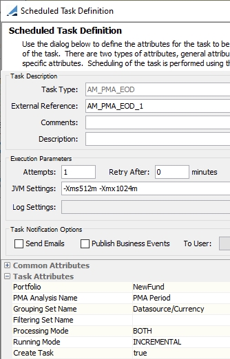
Task Attributes:
| • | Portfolio – Id or name of the Grouping Hierarchy Portfolio to be used at the analysis entry point. |
| • | PMA Analysis Name – Select an Analysis Server Configuration which has been defined for a PMA analysis. |
| • | Grouping Set Name – Name of the grouping set employed to organize and aggregate portfolio positions. Select one grouping by task execution, in combination with the Incremental running mode to historize the data linked to multiple grouping configurations. |
| • | Filtering Set Name – Filtering set (applicable context) to be applied for PMA Daily analysis historization. |
| • | Processing Mode – Select the desired processing mode: |
| – | DAILY_ONLY: Used for PMA Daily data consistency validation. This mode only stores the PMA Daily reports in the Time Series Data Warehouse as PMA Period reports. When the task is run in this mode, you will not be able to launch the consolidated final PMA analysis. |
| – | PERIOD_ONLY: This mode only stores the PMA Period reports in the Time Series Data Warehouse. The task must have been run previously in DAILY_ONLY mode in order to use PERIOD_ONLY mode. PERIOD_ONLY mode allows you to display the final consolidated PMA analysis. |
| – | BOTH: Executes in order the previous configuration. |
| • | Running Mode – Select INCREMENTAL for incremental updates only, or OVERRIDE to overwrite all existing results for the specified parameters. SIMULATE is not supported. |
| • | Create Task – Select true to create a task when an exception occurs (default), or false otherwise. |
Ⓘ [NOTE: It is not necessary to run AM_PMA_EOD for each date. One run will save data for all the dates of the period specified in the PMA analysis.]
Once the PWS inner configurations are done for the PMA Period and PMA analyses, it is necessary to create an AM_PMA_EOD scheduled task and execute it to generate the final output.
It is not possible to consult any information from the PMA Period or PMA analyses before running the AM_PMA_EOD scheduled task as both analyses depend on historized data stored by this task.
7. Running the PMA Period Analysis
To execute a PMA Period analysis, select an ad-hoc valuation date. The selected date must be congruent with the related PMA execution period.
You may execute each day by modifying the valuation date or run the PMA Period analysis for multiple days using a custom start date. The PMA Period’s intention is to debug possible errors for the final PMA analysis and not to be used as a functional report.
8. Running the PMA Analysis
You can view the results of the PMA analysis in the Portfolio Workstation.
See Portfolio Workstation for information on running the Portfolio Workstation.
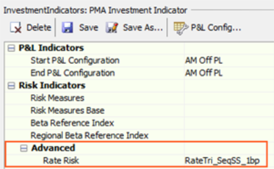
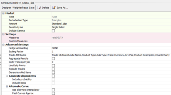
9. Advanced Risk Indicator
For user customized Advance Attribution formulas, the Investment Indicator has an Advance Rate Risk field. A Rate-type Sensitivity configuration can be selected, based on Underlying or Triangles Perturbation Types.
Please refer to Sensitivity documentation for more information about Rate-type Sensitivity, it is strongly recommended that you contact your Calypso representative for configuration advice.
PMA Specific Configuration
Please note the following when configuring PMA analysis in the Portfolio Workstation:
| • | Column Sets – PMA supports Pivot view. The columns DataSource and Period are recommended to be used as pivot columns. |
| • | Groupings – The Grouping must be created with the NODE_ID column and it should be named the same as the column name. |
| • | Layouts – The Default Grouping must be set as the same grouping specified in the AM_PMA_EOD scheduled task. |
Sample PMA Results
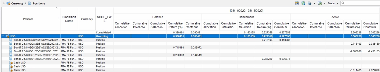
Risk Indicators
Return Std Dev (%) = A measure of the average deviations of a return series from its mean. A large standard deviation implies that there have been large swings or volatility in the manager’s return series.
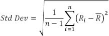
where
Ri is the return for the period i
R is the average return of the overall period
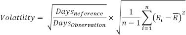
Return Vol (%) = Annualized standard deviation
Tracking Error = The amount of active risk being taken by a manager. Computed by subtracting the return of a specified benchmark or index from the manager’s return for each period, and then calculating the standard deviation of those differences. A higher tracking error indicates a higher level of risk, not necessarily a higher level of return, being taken relative to the specified benchmark. Tracking error only accounts for deviations away from the benchmark, but does not signal in which directions these deviations occur (positive or negative).
![]()
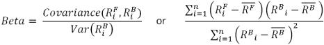
where
RFi is the return of the fund for the period i
RF is the average return of the fund on the overall period
RBi is the return of the benchmark for the period i
RB is the average return of the benchmark on the overall period
Beta (%) = A measure of a portfolio’s volatility. Statistically, beta is the covariance of the portfolio in relation to the market. A beta of 1.00 implies perfect historical correlation of movement with the market. A higher beta manager will rise and fall more rapidly than the market, whereas a lower beta manager will rise and fall more slowly. For example, a 1.10 beta portfolio has historically been 10% more volatile than the market.
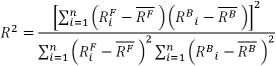
Determination Coefficient = A measure of a manager’s movement in relation to the market. Generally, the R2 of a manager versus a benchmark is a measure of how closely related the variance of the manager returns and the variance of the benchmark returns are. In other words, the R2 measures the percent of a manager’s return patterns that are “explained” by the market and ranges from 0 to 1. For example, an R2 of 0.90 means that 90% of a portfolio’s return can be explained by movement in the broad market (benchmark).
Sharpe Ratio = This statistic is computed by subtracting the return of the risk-free index (typically 91-day T-bill or some other cash benchmark) from the return of the manager to determine the risk-adjusted excess return. This excess return is then divided by the standard deviation of the manager. A manager taking on risk, as opposed to investing in cash, is expected to generate higher returns and Sharpe measures how well the manager generated returns with that risk. In other words, it is a measurement of efficiency utilizing the relationship between annualized risk-free return and standard deviation. The higher the Sharpe Ratio, the greater efficiency produced by this manager. For example, a Sharpe Ratio of 1 is better than a ratio of 0.5.
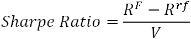
where
RF is the annualized return of the fund over the period
Rrf is the annualized risk-free rate over the period
V is the annualized volatility of the fund over the period
Treynor Ratio = Similar to the Sharpe Ratio, this statistic is computed by subtracting the return of the risk-free index (typically 91-day T-bill or some other cash benchmark) from the return of the manager to determine the risk-adjusted return. This excess return is then divided by the Beta of the portfolio. This is another efficiency ratio that evaluates whether the manager is being rewarded with additional return for each additional unit of risk being taken with risk being defined by Beta, a measure of systematic risk, not Total Risk (standard deviation).
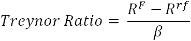
where
RF is the annualized return of the fund over the period
Rrf is the annualized risk-free rate over the period
β is the beta of the fund over the period
Information Ratio = This statistic is computed by subtracting the return of the market from the return of the manager to determine the excess return. The excess return is then divided by the standard deviation of the excess returns (or Tracking Error) to produce the information ratio. This ratio is a measure of the value added per unit of active risk by a manager over an index. Managers taking on higher levels of risk are expected to then generate higher levels of return, so a positive IR would indicate “efficient” use of risk by a manager. This is similar to the Sharpe Ratio, except this calculation is based on excess rates of return versus a benchmark instead of a risk-free rate.
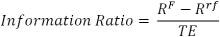
where
RF is the annualized return of the fund over the period
Rrf is the annualized risk-free rate over the period
TE is the beta of the fund over the period
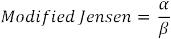
Modified Jensen = Modified Jensen’s alpha is Jensen’s alpha divided by beta.
Skewness = Skewness characterizes the degree of asymmetry of a distribution around its mean. Positive skewness indicates a distribution with an asymmetric tail extending toward more positive values. Negative skewness indicates a distribution with an asymmetric tail extending toward more negative values.
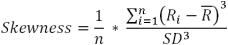
where
Ri is the return for the period i
R is the average return of the overall period
SD is the standard deviation
n is the number of returns
Kurtosis = Kurtosis characterizes the relative peakedness or flatness of a distribution compared with the normal distribution. Positive kurtosis indicates a relatively peaked distribution. Negative kurtosis indicates a relatively flat distribution. If there are fewer than four data points, or if the standard deviation of the sample equals zero, Kurtosis returns the N/A error value.
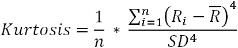
where
Ri is the return for the period i
R is the average return of the overall period
SD is the standard deviation
n is the number of returns
Jarque Bera Test

Downside Deviation = A measure of the average deviations of a negative return series. A large downside risk implies that there have been large swings or volatility in the manager’s return series when it is below the selected hurdle rate (MARR). Downside deviation (also known as downside risk) attempts to further break down volatility between upside volatility, which is generally favorable since it implies positive out-performance, and downside volatility, which is generally unfavorable and implies loss of capital or returns below an expected or required level.
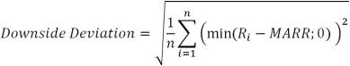
and

where
Ri is the return for the period i
n is the number of returns
MARR is the Minimum Acceptable Rate of Return. Must be entered manually in the Performance Measurement analysis.
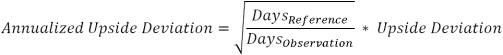
DaysReference is the number of days of reference for a period
DaysObservation is the number of days of sub-periods (1 for daily, 5 for weekly open days, for instance)
Upside Deviation = The standard deviation of all positive returns.
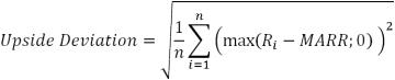
and
where
Ri is the return for the period i
n is the number of returns
MARR is the Minimum Acceptable Rate of Return. Must be entered manually in the Performance Measurement analysis.
DaysReference is the number of days of reference for a period
DaysObservation is the number of days of sub-periods (1 for daily, 5 for weekly open days, for instance)
Sortino Ratio = This measure is very similar to the Sharpe Ratio except that it is concerned only with downside volatility (unfavorable) versus total volatility (both favorable, upside volatility and unfavorable, downward volatility). This statistic is computed by subtracting the return of the risk-free index (typically 91-day T-bill or other cash index) from the return of the manager to determine the risk-adjusted excess return. This excess return is then divided by the downside risk of the manager. A manager taking on risk, as opposed to investing in cash, is expected to generate higher returns and Sortino measures how well the manager “spends” that risk, while not penalizing them for upside volatility (out-performance). The higher the Sortino Ratio, the better; a Sortino Ratio of 1 is better than a ratio of 0.5 – higher excess return and/or lower downside risk.
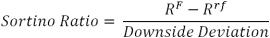
where
RF is the annualized return of the fund over the period
Rrf is the annualized risk-free rate over the period
Downside Deviation is the annualized downside deviation
Performance Indicators
Return Best Period = Period from the rolling period with the highest return. Computed at fund and benchmark level.
Return Worst Period = Period from the rolling period with the worst return. Computed at fund and benchmark level.
Positive Return (%) = Percentage of periods with strictly positive returns. Computed at fund and benchmark level.
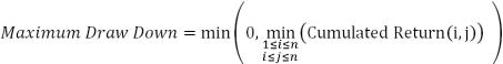
Return Max Loss (%) = Lowest cumulative return in the period as if an investor had subscribed at the beginning of the period and sold their share at the worst time.

where
n is the number of daily periods during the considered period
Cumulated Return(1,i) is the cumulative return from the start of the first daily period to the end of the daily period i
Return Max Draw Down (%) = Lowest cumulative return in the period as if an investor had subscribed and sold their share at the worst time.
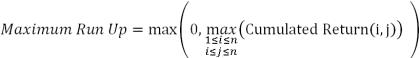
Return Max Run Up (%) = Highest cumulative return in the period as if an investor had subscribed and sold their share at the best time.
Contribution To Vol (%) = Decomposition of volatility contribution at the holding level. You need to add a grouping by Product Description to have it at the holding level.
ContributionToVol = Std Dev(PositionContributions) * Correl(PositionContributions,PortfolioReturns) * SQRT(BaseDays)
Contribution To Tracking Error (%) = Decomposition of tracking error at the holding level. You need to add a grouping by Product Description to have it at the holding level.
ContributionToTrackingError = Std Dev(ActiveContributions) * Correl(ActiveContributions,PortfolioReturns) * SQRT(Base Days)
MW Annualized Return (%) = Modified Dietz money weighted return for a period shorter than 1 year.

where y is number of years, and > 1
Campisi Fixed Income Performance Attribution
Campisi performance attribution considers the unique factors of bond performance, and provides a further decomposition of the Local and FX returns of fixed income products.
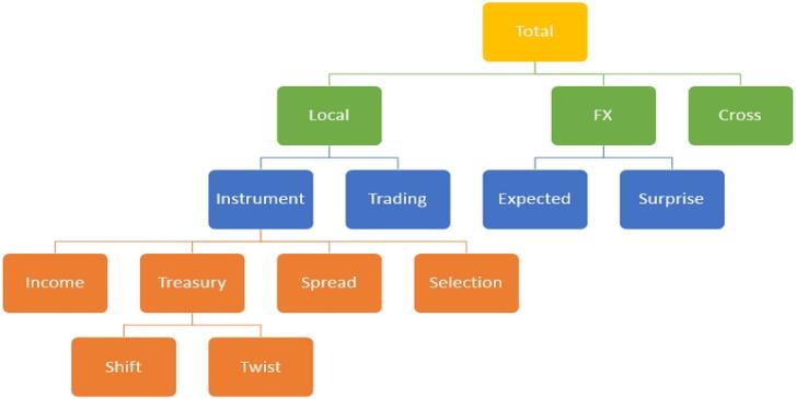
The effects shown in the decomposition diagram above are calculated as follows:
Instrument
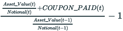
Income
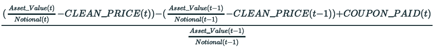
Treasury
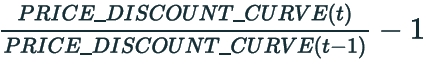
where
PRICE_DISCOUNT_CURVE is the price using discount curves only (no quotes and no credit curves)
Ⓘ [NOTE: In addition to curve movements, it takes Roll Down and Pull-to-par effects into account.]
Shift

where
5Y is the curve point specified in the Campisi Parallel Shift Point analysis parameter - this value can be changed
Twist = Treasury - Shift
Spread
The Spread calculation depends on the value of the Campisi Spread Source analysis parameter.
| Campisi Spread Source value | Calculation |
|---|---|
| Residual |
All positions Spread = Instrument - Treasury - Income |
| Benchmark Sector |
Benchmark positions Spread = Instrument - Treasury - Income Portfolio positions in sectors that exist in the benchmark See below. Portfolio positions in sectors that do not exist in the benchmark Spread = Instrument - Treasury - Income Ⓘ [NOTE: This scenario was not anticipated by Campisi as a portfolio manager would normally not be investing in a sector not contained in the benchmark.] |
Portfolio positions in sectors that exist in the benchmark
| • | Compute the implied Spread change for this sector in the benchmark: |

where

| • | Compute the Spread Return induced by the Spread Change: |

Selection = Instrument - Treasury - Income - Spread
| • | If analysis parameter Campisi Spread Source = Residual, it should always be 0. |
| • | If analysis parameter Campisi Spread Source = Benchmark Sector, it should be 0 for the benchmark. |
Trading = Local - Instrument
Any Local return that doesn't come from the Instrument itself is a Trading return.
Expected FX
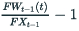
where
FW is the forecast FX rate from the FX curves
FX is the FX spot rate
Surprise FX = Total FX - Expected FX
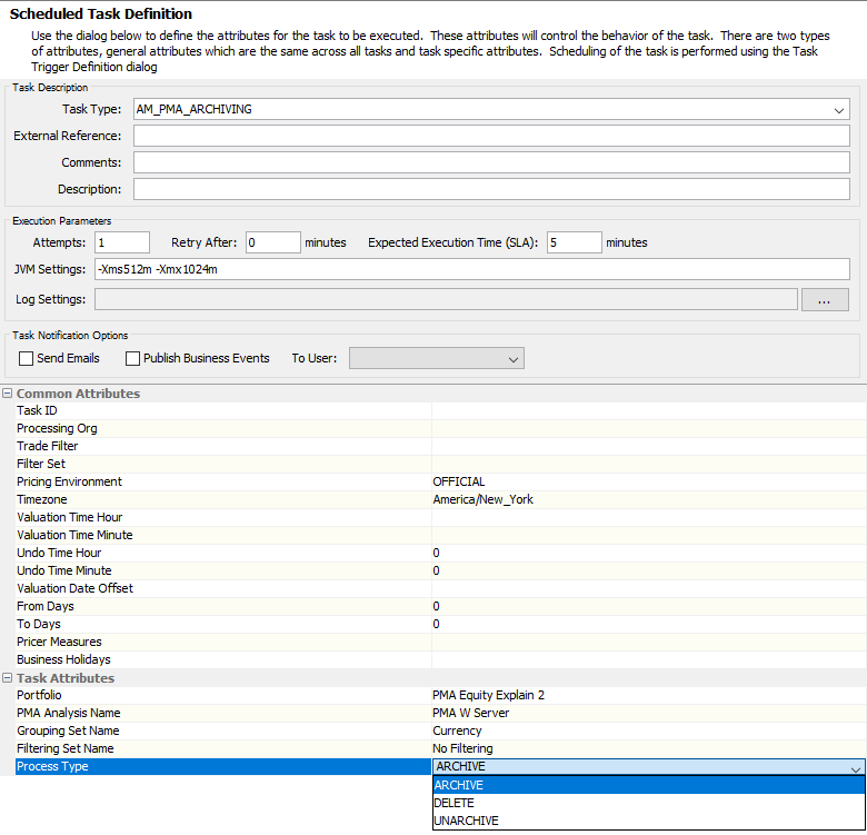
10. AM_PMA_ARCHIVING scheduled task
AM_PMA_ARCHIVING ST scheduled task can ARCHIVE or UNARCHIVE the timeseries data that migrates from timeseries tables in BSDW to hist timeseries tables in BSDW.
Task Attributes:
-
Portfolio – Name of the Portfolio to be used at the analysis entry point.
-
PMA Analysis Name – Select a Analysis Server Configuration which has been defined for a PMA analysis.
-
Grouping Set Name – Name of the grouping set employed to organize and aggregate portfolio positions. Select one grouping by task execution, in combination with the Incremental running mode to historize the data linked to multiple grouping configurations.
-
Filtering Set Name – Filtering set (applicable context) to be applied for PMA Daily analysis historization.
-
Process Type:
-
ARCHIVE: Migrates a PMA dataset from timeseries tables in BSDW to hist timeseries tables in BSDW. The corresponding PMA data is not available to consult on PWS after archiving.
-
ARCHIVE: Retrieves a PMA dataset from hist timeseries tables in BSDW to timeseries tables in BSDW. The corresponding PMA data would be available to consult on PWS after archiving.
-
DELETE: Currently is not supported.
-