Simulation
Simulation allows reporting on the impact to pricing results of broad shifts to market data and to the time horizon.
Overview
Simulation allows configuring market data combinations to be shifted, and shift amounts in an intuitive way. Depending on the market data item, the shift can be defined as parallel or non-parallel.
Where a market data item is made up of many underlying elements or instruments, the rates for all elements will be shifted simultaneously.
Where more than one piece of market data are shifted in combination (for example, the FX Spot rate and a zero curve), then both will be shifted simultaneously and the trades or positions re-priced.
Simulation can be configured from Configuration > Reporting & Risk > Analysis Designer. Right-click a Simulation folder (for example, 'Favorites') in Analysis Designer, and choose 'New Analysis' to add a parameter configuration, you will be prompted to enter a configuration name.
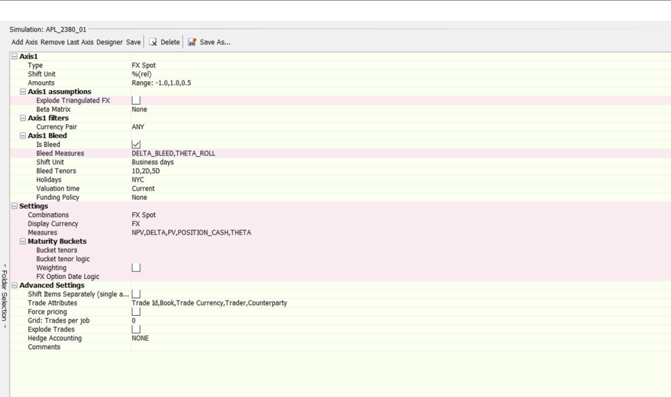
Sample Simulation parameters
| » | Complete the parameter details. They are described below. |
| » | Click Save to save the configuration. |
Simulation results can be viewed in the Calypso Workstation.
 Refer to Calypso Workstation documentation for setup details.
Custom Pricer Measures
NOTE: Custom Pricer Measures which require market data in addition to what is already managed by the Pricer are not supported (e.g. ACCURAL_BO_BASE, VEGA_BASE). Any “Base” conversions can be configured to occur at report level.
1. Simulation Parameters
Each Simulation parameter consist of one or more axes. Each axis defines the type of market data item being shifted, how the shift will be applied and the magnitudes of the shifts. For each parameter, five axes can be defined.
Each parameter also contains Settings and Global Assumptions. Settings define globally for all the axes in the parameter how the Simulation analysis results will be displayed, which measures to include in the pricing and if the axes will be run individually or as combinations.
Global Assumptions define which additional trade or product information will be included in the output as well as some advanced definition regarding how this analysis will be run.
Ⓘ [NOTE: The following settings are limited to prevent running into memory and performance issues]
| • | No more than 30 trade attributes |
| • | No more than 20 underlier attributes |
| • | Cannot select more than 20 pricer measures |
| • | Cannot compute more than 500 pricer measures per trade overall (number pf pricer measures * number of shifts / axis * number of axes) |
1.1 Simulation Types
The following axes are available.
| Types | Description | |||||||||
|---|---|---|---|---|---|---|---|---|---|---|
|
FX Spot |
The FX Spot Simulation shifts direct and triangulated FX Spot Quotes by a defined number of pips or by a percentage of spot. In its simplest form, it creates a spot ladder up and down from current spot in your chosen increments. The intention is to run the FX Spot axis independently to provide a spot ladder or in combination with FX Volatility, a Rate axis or Time Horizon simulation to build an array of simulated conditions at which trades and positions are priced. This will then provide a matrix of exposure and values that can be interrogated and analyzed. Many products have FX exposure. However, the featured use case for this simulation is for an FX or FX derivatives book.
|
|||||||||
|
Rate |
The Rate Simulation allows the user to calculate the changes in NPV or other Pricer Measures due to shifts on the Zero and/or Basis Curves, depending on the Shift Items Separately setting. The Rate Simulation shifts all curve output points simultaneously by the size of shift specified by the user. Alternatively, the user can apply shifts of different sizes for user-defined buckets using the non-parallels feature inside of the Scenario – Measure Maker window and applying this as a Custom shift. You can also shift Product Specific interest rate curves by adding their usage to the domain "ScenarioMarketDataSet.Rates" - Example: FWD_PRICE_FOR.
|
|||||||||
|
Yield |
The Yield Simulation allows computing changes on NPV due to shifts in the Yield curves. |
|||||||||
|
Volatility |
BOND Volatility The BOND Volatility Simulation shifts the BOND Volatility Surface. It simultaneously shifts all the points on the BOND volatility surface. COMMODITY Volatility The COMMODITY Volatility Simulation shifts the COMMODITY Volatility Surface. It simultaneously shifts all the points on the COMMODITY volatility surface. The primary purpose of sliding the volatility is to view the impact of a potential market move on the user's portfolio. CREDIT Volatility The CREDIT Volatility Simulation shifts the CREDIT Volatility Surface. The slide allows the ability perturb the volatility which can be derived from option prices or be directly input by the users. For example, the users may want to quickly see the impact on their portfolio is the credit volatility moved by +10% and -10%. EQUITY Volatility The EQUITY Volatility Simulation shifts the EQUITY Volatility Surface. It simultaneously shifts all the points on the EQUITY volatility surface by a user-defined absolute or relative amount. The amounts can either be a range or custom set of amounts. For example, -5% to 5% by 2.5% absolute. FX Volatility The FX Volatility Simulation applies a uniform, parallel shift to the volatility surface by simultaneously shifting all the points. The shift amounts can be defined by % volatility units or as a relative % of current volatility. Non-parallel shifts are surface not permitted. The intention is to run this independently as a volatility ladder or together with FX Spot, Rate or Simple Horizon simulations to build a matrix of simulated conditions at which exposure or NPV can be calculated. The most important use is clearly for a book that has FX Volatility sensitivity. RATE Volatility The RATE Volatility Simulation allows the user to calculate the changes in NPV or other pricing results due to shifts in the Volatility Surface. The Volatility Simulation simultaneously shifts all volatility points by the shift increments specified by the user. Surface types covered are RATE, BOND OPTION, BOND FUTURE, and MM FUTURE. For surfaces of type RATE, simultaneous point shifts are performed on the principal layer of the surface (Black or BpVol) as determined by the generator and scaled accordingly. |
|||||||||
|
Correlation |
The Correlation Simulation shifts the Correlation Surface, correlation quotes and Correlation Matrix. The simulation allows the ability to perturb the correlation values which can exist on a correlation surface, correlation matrix or a correlation quote. This allows the users to see an impact of correlation movements on the portfolio. For example, the users may want to quickly see the impact on their portfolio if the correlation moved by +10% and -10%. Any Correlation Matrix with more than 3 axes is not supported. |
|||||||||
|
SimpleHorizon |
Simple Horizon simulates moving the valuation date forward by one business day. Specifically it moves the valuation time to 00:00:01 on the following business day. This is a simplified horizon shift using the assumption that no trade events will have taken place yet for the horizon day so simply you are reflecting one day less to maturity for the trade. Simple Horizon can be combined with any of the other axes to form a matrix of simulations. The Simple Horizon simulation is relevant to any product type. |
|||||||||
|
The purpose of this analysis is to provide the user with an estimated NPV of the portfolio as of a Horizon Date and Time. This involves market data rolling, trade lifecycle (option exercise), cash flows, and funding. It currently applies to IRD products (excluding eXSP), FX products, and Equity products, but not for pricing script products. The supported Equity products are Equity Structured Option (with payout Vanilla, underlying Equity or Equity Index, exercise style European only), Future Equity, Future Equity Index, Equity, and Security Lending. All FX products are supported, except for FX Compound Options. The supported IRD products are: Swap, Swap w/Cancellable Extension, Cancellable Swap, CapFloor, CappedSwap, Swaption, FRA, Cash, SpreadCapFloor, SpreadSwap, FutureMM, FutureBond, FutureSwap, FutureMMOption, FutureBondOption, Bond, BondOption, NDS, SwapCrossCurrency, SwapNonDeliverable, and StructuredFlows. Ranges and Curves The Horizon Date Range is defined as the interval between the Valuation Date included and the Horizon date excluded. The user can configure a series of horizon dates based on tenors or specific dates that define the time simulation shifts. The portfolio will be revalued at each horizon date and time using the evolved market data. The difference between the initial and horizon portfolios will be the horizon date (which the horizon portfolio trades will be valued from). The portfolios can be viewed in a trade window or blotter. The way to roll market data forward is defined at each generator’s level. For rate curves however the rolling method is overridden and the “roll forward” is applied regardless of the configuration:
Assumptions are pre-defined for lifecycle behavior of the supported products during the time to the horizon. TimeHorizon will check the option for all possible exercise dates (once for European, a few times for Bermudans, all dates for American). The option will be exercised as soon as it is in the money. For Bermudan and American options, that can lead to exercise not at the optimal date, but still valid. Funding All cashflows are funded from the date they fall on until the Horizon Date. Funding is specified according to funding policy and cashflow currency. Retrieve the cashflows by using the dedicated funding curve. In the pricer config window, click the "Product Specific" tab and select TIME_HORIZON_FUNDING from the drop down menu in "Usage." Funding policies can be set as 'none', 'Horizon', 'Daily' or customized by users through an API. The Time Horizon Simulation can be run in combination with the other Simulation types (for example Time Horizon by FX Spot). In these cases the direction is always that the market data simulation is performed first and the Time simulation second. Only NPV, HORIZON_CASH and HORIZON_FUNDING are validated in Time Horizon Analysis::
|
||||||||||
|
Commodity |
The Commodity Simulation shifts the Commodity Forward Curve. The Commodity Forward Curve can be shifted in a parallel or non-parallel manner. The simulation shifts each commodity curve underlying by a specified number of basis points or by a percentage of the price. In commodity terms, one basis point has always equaled a price movement of 0.01 in the currency of the commodity. The primary purpose of sliding the forward price is to view the impact of a potential market move on the user's portfolio. |
|||||||||
|
Equity |
The Equity Simulation shifts Equity Quotes (single name and index). The simulation shifts the quotes by a defined percentage. The amounts can either be a range or custom set of amounts. For example, -5% to 5% by intervals of 2.5% absolute. If a Beta Reference Index is specified for the simulation, the shifts for each asset will be scaled by its respective Beta to the index. For example, given shifts of -5% to 5%, by 2.5%, a Beta: Reference Index of S&P 500, and the asset of GE with a beta of 1.5, GE's shifts will be -7.5% to 7.5% by intervals of 3.75%. The Beta: Reference Index is optional. When the market moves, not all assets in a portfolio increase or decrease their rates of return by the same amount. The Beta indicates the correlation of the asset’s rate of return and the market’s rate of return. The market is represented by an index, such as the S&P 500 and is assigned a Beta of 1.0. If the market’s rate of return increases by 1%, and a stock’s rate of return increases by 3%, then the stock has a Beta of 3.0. |
|||||||||
|
Dividend |
The Dividend Simulation shifts the Dividend Curve. The simulation shifts the points on the dividend curve by the defined percentage. |
|||||||||
|
Borrow |
The Borrow Simulation shifts the Borrow Curve. The Borrow Curve typically is represented as a spread relative to a zero yield curve. The shifts can either be absolute in bps or percent, or relative percentage. |
|||||||||
|
Credit |
The Credit simulation shifts the credit spread and credit quotes. The simulation allows the ability perturb the credit spreads which can be used to build a curve or specified as a quote. This allows the users to see an impact of the credit movements on their portfolio. For example, the users may want to quickly see the impact on their portfolio is the credit spreads moved by +10% and -10%. The credit simulation allows the ability to see the systemic risk (shifting all the curves) or idiosyncratic risk (impact of a specific curve). |
|||||||||
|
Recovery |
The Recovery Simulation shifts the Recovery Rate specified on each Probability Curve of the portfolio. After each shift, the corresponding Probability Curve is then regenerated and used to price any related trades. This allows the users to see an impact of the Recovery Rate movements on their portfolio. For example, users may want to quickly see the impact on their portfolio if the Recovery Rate moves by +10% and -10%. The Recovery slide report allows the ability to see the systemic risk (shifting all the curves) or idiosyncratic risk (impact of a specific curve). |
|||||||||
|
Prepayment |
The Prepayment Simulation is either a relative percentage shift or an absolute amount shift in the Prepayment Curve. If the absolute amount shift is employed, the units match the units used in the Prepayment Curve being shifted. Prepayments are early amortization of principal of a mortgage backed security caused by the mortgagor(s) partially or completely repaying the debt earlier than the scheduled amortization. In typical mortgage backed securities, increased prepayments cause an increase in earlier cash flows, thus a shorter average life and other resultant changes in all cash flow analytics. |
|||||||||
|
Default |
The Default Simulation shifts the Default Curve for ABS (asset-backed securities) bonds. The simulation shifts the points on the default curve by the defined percentage. |
|||||||||
|
Inflation |
The Inflation Simulation shifts the Inflation Curve. Any product that involves future cash flows linked to inflation indexes are subject to inflation curve perturbations (for example, bonds and swaps). |
1.2 Axis Parameters
Select the type of simulation from the Type field.
For Volatility or Correlation simulations, you can also choose the Volatility Type or Correlation Type.
In case you have implemented custom volatility types, you can add the volatility types to domain "simulationCustomVolatilityType" as needed.
Once the Type is selected, the Shift Unit can be selected.
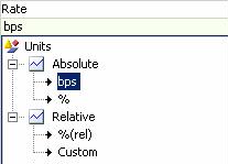
Depending on the type of simulation, the market data can be shifted in terms of basis points, pips, dollar amounts, cents amounts, absolute or relative percentage, or business days:
| • | One basis point is one-hundredth of a percent. Basis point shifts can be applied to zero yield curves, basis curves, dividend curves, borrow curves, credit curves, and inflation curves. |
| • | A pip is used in foreign exchange rates. This follows market convention, and this convention is defined elsewhere in the system per currency pair. For example, in the pair EUR/USD, a pip is equal to 0.0001 (i.e. if the EUR/USD exchange rate is 1.5000, then an increase of one pip would bring the exchange rate up to 1.5001). |
| • | Relative percentage shifts can be applied to All rate types while absolute percentage shifts can be applied to market data that is itself defined as a percentage. |
| • | Shifts of dollar or cents amounts can be applied to commodity forward curves. |
| • | Calendar or business day shifts are used with the Time Horizon axis. |
After the Shift Unit is chosen, the amount to be shifted can be entered from the Amounts field.
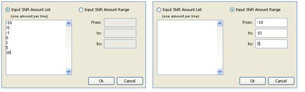
The user has two options for entering shift amounts. The Input Shift Amount List can be selected and specific amounts entered, with one amount per line.
If the shift amounts come in evenly spaced intervals, then the Input Shift Amount Range can be used. The user can enter the minimum and maximum value of the range, and the interval between different shift amounts. In this example, the range goes from -10 to +10 in intervals of 5, so the shift amounts will be -10, -5, 0, 5, and 10 bps (basis points).
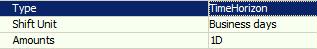
For Time Horizon, the shift unit is business days or calendar days, and the amounts are the tenors that define the horizon dates.
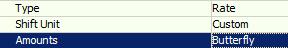
Custom Shift Unit
Where it is available for an axis, selection of the Custom shift unit will allow you to select one or more pre-defined non-parallel shift configurations. The non-parallel shift configurations can map to different shift amounts for different maturity buckets within one simultaneous market data shift item shift.
Click Designer to define non-parallel shifts. The Scenario – Measure Maker window will open.
See Analysis Designer - Measure Maker for details.
1.3 Axis Assumptions
The items under "Axis assumptions" will differ based on the Axis Type.
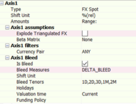
FX Spot
Explode Triangulated FX
Check to explode the sensitivity of a currency pair by triangulation currency, or clear to ignore the triangulation currency. This option has no effect on currency pairs that are not triangulated.
Triangulation currencies are defined in a triangulation rule using Configuration > Definitions > Triangulation Ccy Rule Set. The triangulation rule is set in the pricing parameter TRIANGULATION_CCY_RULESET_NAME.
For example, the currency pair EUR/CHF is triangulated using the USD currency.
If "Explode Triangulated FX" is checked, the report will show the sensitivity to EUR/USD and the sensitivity to USD/CHF.
If "Explode Triangulated FX" is not checked, the report will show the sensitivity to EUR/CHF.
Refer to Calypso FX documentation for details on these settings.
Beta Matrix
Beta matrices allow selecting a "parent" currency pair for a family of currency pairs. The members of the family are related to the parent via the Beta factor. Shifts to the parent and unrelated pairs will be defined in the FX Spot axis. Shifts to the family members will be the reference shifts scaled by the Beta factor for each currency pair defined as "related".
The definition of the Betas between currency pairs is made in Market Data > Correlation & Covariance > Beta Value.
Simple Horizon
You can select:
| • | Holidays - Select the holiday calendar to determine which days will be considered business days when shifting the valuation time. |
| • | Whether to roll quotes or not - We do not know what the quotes are for a future date. Therefore you can set this parameter to TRUE (the default setting) to use the current quotes for valuation of trades at the horizon date as well. |
Time Horizon
You can select:
| • | Holidays - Select the holiday calendar to determine which days will be considered business days when shifting the valuation time. |
| • | Valuation time |
| • | Funding policy: none or horizon (use forward rate from cash flow rate until horizon date). |
The "horizon" policy requires the setup of a funding curve per currency in the Pricer Config, using the Product Specific tab, usage TIME_HORIZON_FUNDING (for no specific product).
Equity
You can select:
| • | Beta: Reference Index - Choose the Equity Index that will be the reference for computation of any Beta adjusted calculations. |
| • | Underlier Attributes - Attributes on the market data. |
Dividend, Borrow, Credit, Recovery
You can select Underlier Attributes (attributes on the market data).
1.4 Axis Filters
Not all analyses have "Axis filters". The axis filter is a criteria that allows filtering the displayed data.
FX Spot "Axis filter"
You can select one or more currency pairs, or ANY (no filter).
Rate, Commodity, Dividend, Credit, Recovery, Inflation "Axis filter"
You can select one or more currencies, or ANY (no filter).
1.5 Bleed
Bleed enables the computation of Delta Bleed and/or Theta Roll measures based on multiple time horizon tenors and shifts in FX Spot quotes. Users may specify these tenors and Spot shifts as per below guidelines.
Bleed Tenors
-
Tenor specifies by the user. Example 0D, 2D, 1W
-
Time horizon tenors by the user, such as 0D, 2D, 1W
Ⓘ NOTE: Due to performance reasons, the allowed number of tenors is up to 5.
Formula:
Delta Bleed_FX Spot[(x%)]_(n days) = Delta_FX Spot[(x%)]_(n days) – Delta_FX Spot[(x%)]_Delta (0 days)
Theta Roll_FX Spot[(x%)]_(n days) = NPV_FX Spot[(x%)]_(n days) – NPV_FX Spot[(x%)]_Delta (0 days)
"n days” represents the horizon date forward.
“FX Spot[(x%)]” represents the shifted FX Spot.
Ⓘ NOTE: No multi-axis combinations supported for Bleed; the FX Spot Simulation with Bleed can only be run as a single-axis analysis.
1.6 Settings
Settings apply to all types of axes.
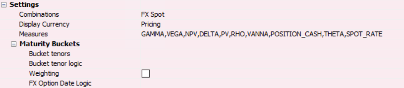
Combinations
Combinations will be significant in a multiple-axis analysis. The user can decide to generate the analysis as combinations of the axes or as separate axes or both.
There is a limit to only allowing two dimensional combinations unless one dimension is a Horizon axis. If so, three will be allowed.
Display Currency
The Display Currency dropdown has two options: Pricing and FX.
If Pricing is chosen, the analysis output will be displayed in the currency in which the pricer returns the measures.
If FX is chosen, the analysis output will be displayed in the currency pair’s “Delta Display Ccy” or “PL Display Ccy” depending on the pricer measure. Delta, Gamma, and Vanna measures follow the “Delta Display Ccy”. PV, NPV and Vega measure follow “PL Display Ccy”.
Measures
Measures are pricer measures that are supported by the product, for example, NPV. Multiple measures can be selected. It is important to note that in an analysis with multiple axes, different measures cannot be selected for each axis. If the user must select different measures for each axis, then separate simulations should be created.
Note: Risk Measures (i.e. equityDELTA, rateDELTA, etc.) can only be run on single axis Simulations and without Shift Items Separately.
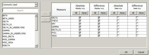
In the Measures window, the user can select how the measure values will be calculated in the analysis.
The “Absolute (display ccy)” output shows the NPV as an absolute value in terms of the trade currency, while the “Absolute (base ccy)” output shows the NPV as an absolute value in terms of the base currency of the user.
The “Difference (display ccy)” output shows the difference between the NPV resulting from the zero-shift and the NPV resulting from the specific basis point shift in the trade currency. “Difference (base ccy)” shows the same thing in the user’s base currency.
The "Commonly Used" measures are listed for convenience. This list is defined in the domain "SimulationCommonMeasures". You can modify this domain as needed. All measures are accessible by selecting 'Others' in the dropdown menu, not "Commonly Used".
Maturity Buckets
Maturity buckets can be defined. This will prompt the calculation of additional information that can assign the results to the defined buckets. This assignment will use the product maturity date to compare to the bucket dates.
| • | Bucket Tenors: Only enter soft tenors, no hard dates. |
| • | Bucket Holiday Logic: Use holidays from the trade, use the FX spot date, or use specific holidays. |
| • | Weighted Buckets: If checked, each trade will be split appropriately between buckets based on time weighting of the reference date compared to the previous and next bucket dates. If not checked, the trade will fall into the maturity bucket only. |
| • | FX Option Date Logic: Can be relevant in FX Options reporting to bucket by the expiry date in some cases and by delivery date in others. You can define which date to use for maturity bucket purposes. The options are 'Expiry Date' or 'Delivery Date'. |
1.7 Advanced Settings
Advanced Settings apply to all types of axes.
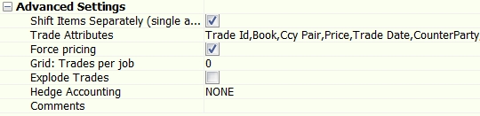
You can set the following parameters:
| » | Shift Items Separately: Determines whether the market data items will be shifted separately or altogether. |
| – | The Shift Items Separately feature is only applicable when one axis is defined. Having more than one axis will force the setting to be False. |
| – | If False, CurveBasis type curves will be skipped to avoid a double counting of the risk. |
| » | Trade Attributes: What trade attributes will appear in the analysis output. |
| » | Force Pricing: Whether all trades that the analysis is applied on will give results. |
| – | If True is selected, then all trades that the analysis, even those that are not sensitive to the market data shift, will have NPVs calculated and displayed in the analysis results. |
| – | If false, only the trades sensitive to the market data shift will have NPVs calculated and displayed in the analysis results. |
| » | Grid: Trades per job: It is possible to run an analysis using a grid of calculators. When doing so, the entire job is broken up into smaller jobs -- each of these smaller jobs can be dispatched to the grid of calculators. The trades per job helps determine how large each job should be. Default is 500. |
| » | Explode Trades: Whether structured trades will be broken down into their individual underlying components prior to running the report. |
[NOTE: For FX Options, 'Explode Trades' will separate the premium from the option to get the report for each separately. The currency pair of the premium can be different to that of the option when traded with a third currency premium. The risk against each currency pair is calculated separately, hence the "exploded" components.]
| » | Hedge Accounting - Select a Participation Classification as needed. It allows grouping hedging trades and hedged trades in the output. Participation Classifications are set in Hedge Definitions. |
Please refer to Calypso Hedge Accounting documentation for details.
| » | Comments: Add any necessary comments for the parameter. |
1.8 Quoted Products
Listed products (example Future Money Market – Calypso product FutureMM) are priced typically from market quotes. However, there is a need to compute risk on these products versus the same market data as OTC trades, in order to aggregate the risk, verify the hedge, or explain the P&L. For example, with a book of IR Swaps hedged with Futures, it is important that the risk of the Futures is computed on the same curve as the Swaps so that the hedge can be verified.
The listed products can be priced either from the direct quotes or theoretically (i.e. price FutureMM from swap curve). In the context of risk, one could price them theoretically and therefore produce the needed risk. However, that approach leads to prices that are inconsistent with the market (direct quotes).
The preferred approach in Calypso is to compute a Pricer Measure that captures the gap between the market price and the theoretical price. This measure is stored and then used as an additional input when pricing theoretically during the risk process. In case of no shift (i.e. 0bp on rates), one can find the market price again.
This approach is called Pre Processing. It applies to Sensitivity, Simulation, MultiSensitivity, IntradayPL, and the scheduled task PL_GREEKS_INPUT.
Pre Processing settings are directly picked up from the database table SCENARIO_QUOTED_PRODUCT. The algorithm is the following:
For each product in the table:
| • | If the Pricer Parameter “PRICER_PARAMS” in the Pricing Environment (Pricer Param Set) is true |
Then pre process the Pricer Measure given in “PRICER_MEASURE”
End if
End for
The table is populated by default upon installation or upgrade.
You can view the content of the table SCENARIO_QUOTED_PRODUCT in the Measure Maker window of Analysis Designer.
|
PRODUCT_NAME |
PRICER_PARAMS |
PRICER_MEASURE |
|---|---|---|
|
Bond |
BOND_FROM_QUOTE |
INSTRUMENT_SPREAD |
|
BondAssetBacked |
BOND_FROM_QUOTE |
INSTRUMENT_SPREAD |
|
BondBrady |
BOND_FROM_QUOTE |
INSTRUMENT_SPREAD |
|
BondFRN |
BOND_FROM_QUOTE |
INSTRUMENT_SPREAD |
|
BondMMDiscount |
MMKT_FROM_QUOTE |
INSTRUMENT_SPREAD |
|
BondMMDiscountAUD |
MMKT_FROM_QUOTE |
INSTRUMENT_SPREAD |
|
BondMMInterest |
MMKT_FROM_QUOTE |
INSTRUMENT_SPREAD |
|
BondOption |
BOND_FROM_QUOTE |
PLXG |
|
ETOEquity |
NPV_FROM_QUOTE |
VOLATILITY_SPREAD |
|
ETOEquityIndex |
NPV_FROM_QUOTE |
VOLATILITY_SPREAD |
|
ETOVolatility |
NPV_FROM_QUOTE |
VOLATILITY_SPREAD |
|
FutureBond |
FUTURE_FROM_QUOTE |
INSTRUMENT_SPREAD |
|
FutureCommodity |
FUTURE_FROM_QUOTE |
INSTRUMENT_SPREAD |
|
FutureDividend |
FUTURE_FROM_QUOTE |
INSTRUMENT_SPREAD |
|
FutureDividendIndex |
FUTURE_FROM_QUOTE |
INSTRUMENT_SPREAD |
|
FutureEquity |
FUTURE_FROM_QUOTE |
INSTRUMENT_SPREAD |
|
FutureEquityIndex |
FUTURE_FROM_QUOTE |
INSTRUMENT_SPREAD |
|
FutureFX |
FUTURE_FROM_QUOTE |
INSTRUMENT_SPREAD |
|
FutureMM |
FUTURE_FROM_QUOTE |
INSTRUMENT_SPREAD |
|
FutureOptionBond |
NPV_FROM_QUOTE |
VOLATILITY_SPREAD |
|
FutureOptionDividend |
NPV_FROM_QUOTE |
IMPLIEDVOLATILITY |
|
FutureOptionDividendIndex |
NPV_FROM_QUOTE |
VOLATILITY_SPREAD |
|
FutureOptionEquity |
NPV_FROM_QUOTE |
VOLATILITY_SPREAD |
|
FutureOptionEquityIndex |
NPV_FROM_QUOTE |
VOLATILITY_SPREAD |
|
FutureOptionMM |
NPV_FROM_QUOTE |
VOLATILITY_SPREAD |
|
FutureStructuredFlows |
FUTURE_FROM_QUOTE |
INSTRUMENT_SPREAD |
|
FutureVolatility |
FUTURE_FROM_QUOTE |
INSTRUMENT_SPREAD |
|
ListedFRA |
NPV_FROM_QUOTE |
INSTRUMENT_SPREAD |
|
PerformanceSwap |
BOND_FROM_QUOTE |
PLXG |
|
Warrant |
NPV_FROM_QUOTE |
VOLATILITY_SPREAD |
Bonds, Futures, and Other Derivatives
For these products, it is recommended to pre-process INSTRUMENT_SPREAD. It is computed by solving the shift amount to be applied on the market data (for instance the rate curve or the equity quote) that aligns the theoretical price and market price.
Listed Options
For Listed Options, one can pre-process IMPLIEDVOLATILITY. This is the level of volatility that makes the theoretical price match the market price. Fixing the volatility allows the computation of Delta and Rho. This approach, however, does not allow the computation of Vega. The preferred approach is to pre-process VOLATILITY_SPREAD that is based on the Volatility Surface and its implied volatility.
Other Products
Some Calypso products like BondOption or PerformanceSwap are not directly priced from quotes, but they embed a product that is. In order to trigger the relevant category in P&L Explained by Greeks, it is necessary to add them in the pre-processing table.
2. Sample IRD Simulation Results in Calypso Workstation
Simulation results can be viewed through the Calypso Workstation. Refer to the Calypso Workstation for setup details.
Click Workstation in the Calypso Navigator to bring up the Calypso Workstation.
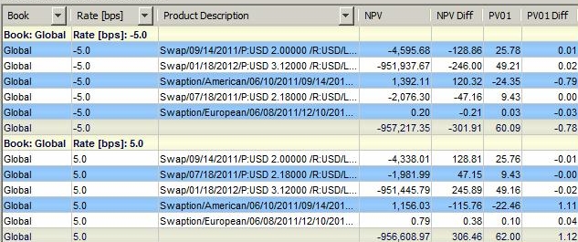
2.1 Example of Simple View
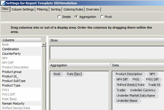
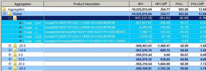
2.2 Example of Aggregation View
The Aggregation view differs from the Simple view in that Aggregation criteria are chosen, and the results are aggregated into folders that are expandable and collapsible.
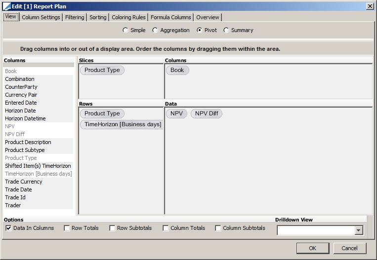
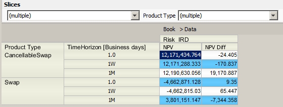
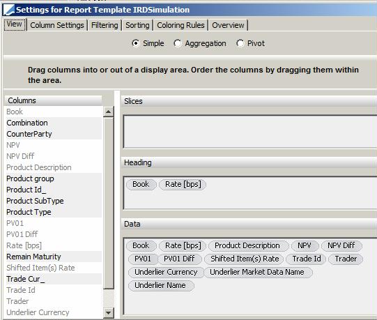
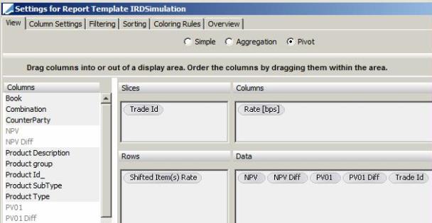
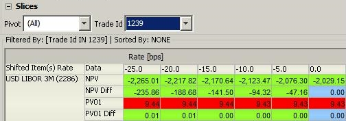
2.3 Example of Pivot View
The Pivot view allows a matrix display. The user can move the items into the different fields in order to get different views of the result display. Sub Totals and Grand Totals can also be chosen for rows and columns in order to display aggregate results.
In the Data Area field, the user will typically put the pricing measure, such as NPV. The shift rules typically go in the Column Area and Row Area. In Slices, the user can put in TradeId, Book, Trade Bundle, or other categorizing items. Every item chosen for Slices will be displayed in an individual dropdown above the pivot table.
3. Sample Time Simulation in Calypso Workstation
Simulation results can be viewed through the Calypso Workstation.
Refer to the Calypso Workstation user guide for setup details.
Click Workstation in the Calypso Navigator to bring up the Calypso Workstation.